library(tidyverse)
library(scales)
library(janitor)
library(glue)
Prison Population and Length of Stay Trends
Introduction
This model code will allow you to produce three data visualizations from the state-specific Justice Data Snapshots, published by The CSG Justice Center. Utilizing the provided model code in the R statistical programming language on your local computer, you will be able to replicate the process of importing data, cleaning and wrangling these data, and finally creating data visualizations displaying prison releases and prison population through bar charts. Additionally, you will use R to create dynamic paragraphs of text that can be inserted into reports.
These original charts and can be found on page 21 of the PDF data snapshots.
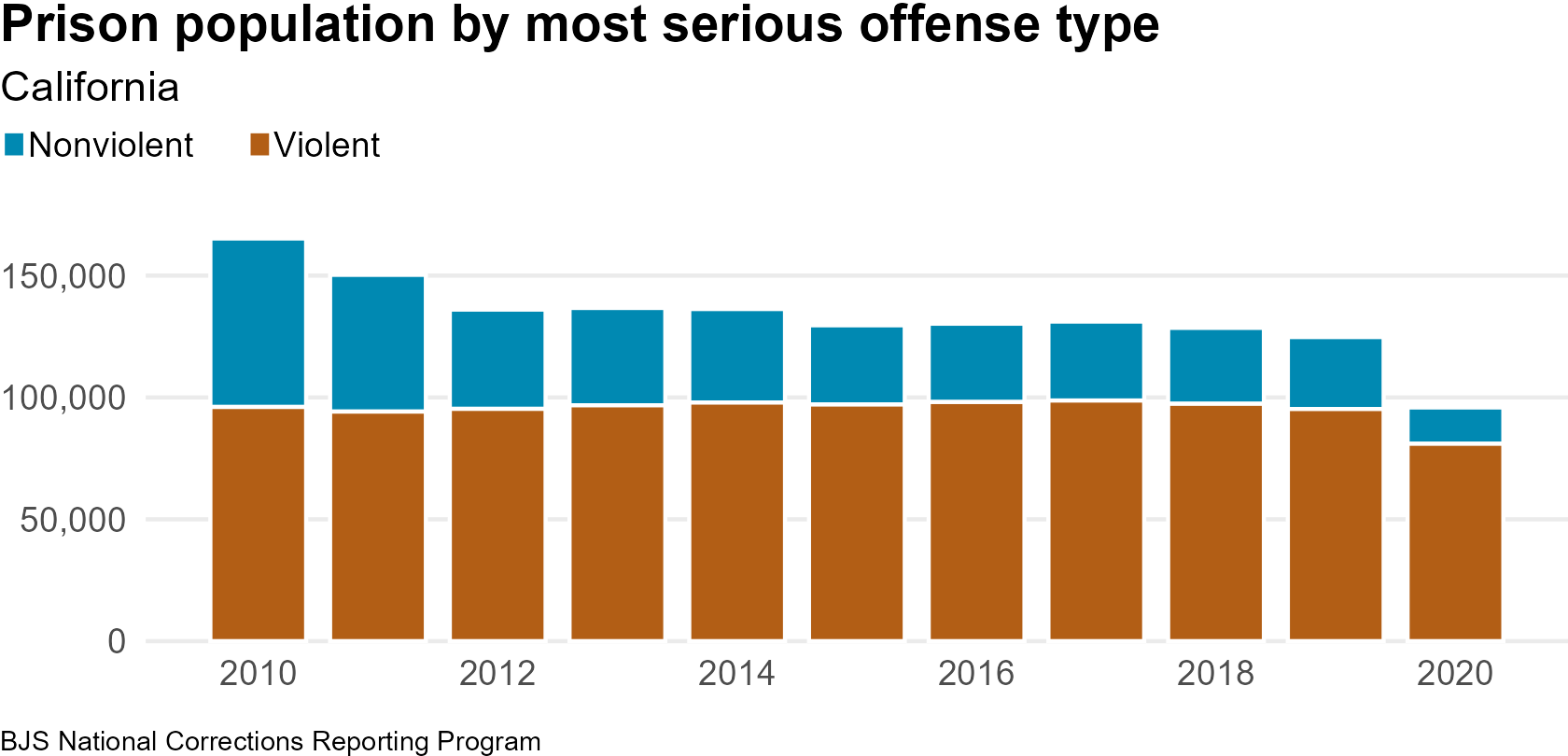
Between 2010 and 2020 in California, the prison population serving sentences for nonviolent offenses decreased by 78 percent, while the prison population serving sentences for violent offenses decreased by 16 percent.
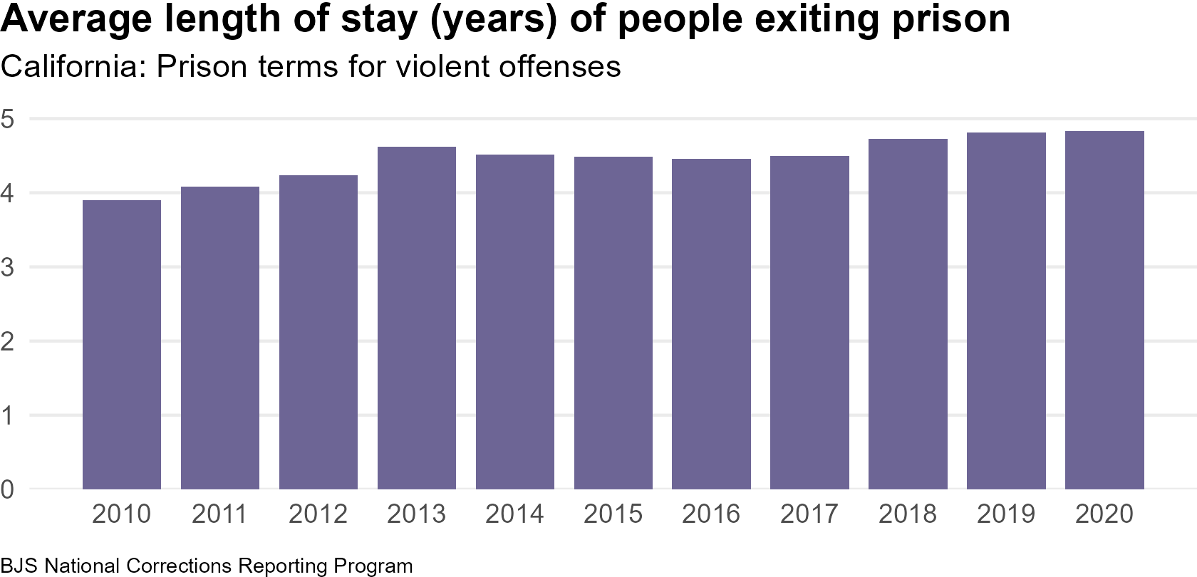
In 2020, the average length of stay of people released from prison who were serving time for a violent offense in California was 4.8 years. This is 4 percent lower than the national average prison stay for violent offenses of 5.0 years.
Load Packages
Prison Population by Most Serious Offense Type
Import Data
The data used for this visualization originally comes from the NCRP Prison Population dataset. If you are interested in downloading the NCRP data and cleaning it yourself, please review Appendix: NCRP Data.
prison_pop_url <- "https://raw.githubusercontent.com/CSGJusticeCenter/va_data/main/model_code/prison_pop_los/state_prison_pop_offense_type.csv"
state_prison_pop_offense_type <- read_csv(prison_pop_url)
#> Rows: 33 Columns: 4
#> ── Column specification ────────────────────────────────────────────────────────
#> Delimiter: ","
#> chr (2): STATE, violent_or_nonviolent
#> dbl (2): RPTYEAR, n
#>
#> ℹ Use `spec()` to retrieve the full column specification for this data.
#> ℹ Specify the column types or set `show_col_types = FALSE` to quiet this message.
this_state <- state_prison_pop_offense_type$STATE[1]
state_prison_pop_offense_type
#> # A tibble: 33 × 4
#> STATE RPTYEAR violent_or_nonviolent n
#> <chr> <dbl> <chr> <dbl>
#> 1 California 2010 Nonviolent 69147
#> 2 California 2010 Violent 96096
#> 3 California 2010 <NA> 56
#> 4 California 2011 Nonviolent 56119
#> 5 California 2011 Violent 94198
#> 6 California 2011 <NA> 163
#> 7 California 2012 Nonviolent 40741
#> 8 California 2012 Violent 95319
#> 9 California 2012 <NA> 144
#> 10 California 2013 Nonviolent 39943
#> # ℹ 23 more rowsCheck Missingness of Data
Some states will have missing offense category data. Because the offense type is missing, these observations cannot be grouped into Violent or Nonviolent categories because we don’t know the original category.
It’s important to review missingness in case it represents a significant amount of the data.
state_prison_pop_offense_type |>
  # calculate total counts per year
  group_by(RPTYEAR) |>
  mutate(total_prison_pop = sum(n)) |>
  # calculate the percentage of missingness for each year
  filter(is.na(violent_or_nonviolent)) |>
  mutate(perc = percent(n/total_prison_pop, accuracy = 0.1))
#> # A tibble: 11 × 6
#> # Groups:   RPTYEAR [11]
#>    STATE      RPTYEAR violent_or_nonviolent     n total_prison_pop perc
#>    <chr>        <dbl> <chr>                 <dbl>            <dbl> <chr>
#>  1 California    2010 <NA>                     56           165299 0.0%
#>  2 California    2011 <NA>                    163           150480 0.1%
#>  3 California    2012 <NA>                    144           136204 0.1%
#>  4 California    2013 <NA>                    700           137425 0.5%
#>  5 California    2014 <NA>                    663           136950 0.5%
#>  6 California    2015 <NA>                    680           130282 0.5%
#>  7 California    2016 <NA>                    396           130667 0.3%
#>  8 California    2017 <NA>                    405           131549 0.3%
#>  9 California    2018 <NA>                    360           128912 0.3%
#> 10 California    2019 <NA>                    348           125132 0.3%
#> 11 California    2020 <NA>                    219            96112 0.2%
All the years of data we are plotting have a missingness of less than 1 percent. Since the missing observations represent such a small percent of the total observations, we are comfortable moving forward and creating the plots.
toplot_state_prison_pop_offense_type <- state_prison_pop_offense_type |>
  drop_na(violent_or_nonviolent)
toplot_state_prison_pop_offense_type
#> # A tibble: 22 × 4
#> STATE RPTYEAR violent_or_nonviolent n
#> <chr> <dbl> <chr> <dbl>
#> 1 California 2010 Nonviolent 69147
#> 2 California 2010 Violent 96096
#> 3 California 2011 Nonviolent 56119
#> 4 California 2011 Violent 94198
#> 5 California 2012 Nonviolent 40741
#> 6 California 2012 Violent 95319
#> 7 California 2013 Nonviolent 39943
#> 8 California 2013 Violent 96782
#> 9 California 2014 Nonviolent 38377
#> 10 California 2014 Violent 97910
#> # ℹ 12 more rowsCreate Plot
Build ggplot
ggplot refers to visual items created using the {ggplot2} package.
gg_prison_population_by_offense <- toplot_state_prison_pop_offense_type |>
  ggplot(aes(
    x = RPTYEAR, # report year on the x-axis
    y = n,  # count of prison population on y-axis
    fill = violent_or_nonviolent, # fill color based on violent or nonviolent
  )) +
  geom_col(width = 0.8, color = "white") + # set the plot type
  scale_fill_manual(values = c("#0089b2", "#b25e15")) + # set the colors
  scale_x_continuous(breaks = seq(2010, 2020, by = 2)) + # set axis breaks
  scale_y_continuous(
    labels = label_comma(1), # style the y labels to include a comma
    expand = expansion(mult = c(0, 0.05)) # remove any add'l spacing on the bottom part of the y-axis
  ) +
  coord_cartesian(clip = "off") + # do not clip the drawing if extends off the plot panel
  labs(
    title = "Prison population by most serious offense type",
    subtitle = this_state,
    caption = "BJS National Corrections Reporting Program",
    x = NULL, # no x axis label
    y = NULL, # no y axis label
    fill = NULL # no lgend label for fill
  ) +
  theme_minimal() + # pre-made themes: https://ggplot2.tidyverse.org/reference/ggtheme.html
  theme(
    plot.title = element_text(
      face = "bold", # make the title font bold
      margin = margin(0, 0, 5, 0) # add margin below title
    ),
    plot.subtitle = element_text(
      size = 11,
      margin = margin(0, 0, 10, 0)
    ),
    plot.caption = element_text(
      size = 7, # set the font size for caption
      margin = margin(10, 0, 0, 0), # add margin at top of caption
      hjust = 0 # make caption left-aligned
    ),
    plot.caption.position = "plot", # align caption to edge of plot
    plot.title.position = "plot", # align title to edge of plot
    axis.text = element_text(size = 9), # increase axis text
    panel.grid.major.x = element_blank(), # remove major grid lines from x-axis
    panel.grid.minor = element_blank(), # remove all minor grid lines from both x and y axis
    plot.margin = margin(1, 0, 0, 0), # remove almost all margin from plot
    legend.position = "top", # put legend at top of chart
    legend.justification = c(0, 0), # pul legend in top left corner
    legend.location = "plot", # align caption to edge of plot
    legend.key.size = unit(7.25, "pt"), # set the size of the boxes in legend
    legend.margin = margin(-5, 0, 5, 0), # specify margin for legend
    legend.box.spacing = unit(10, "pt"),
    legend.text = element_text(
      size = 9, # increase size of legend text
      margin = margin(0, 8, 0, 0) # set legend text margin
    ),
  )
gg_prison_population_by_offense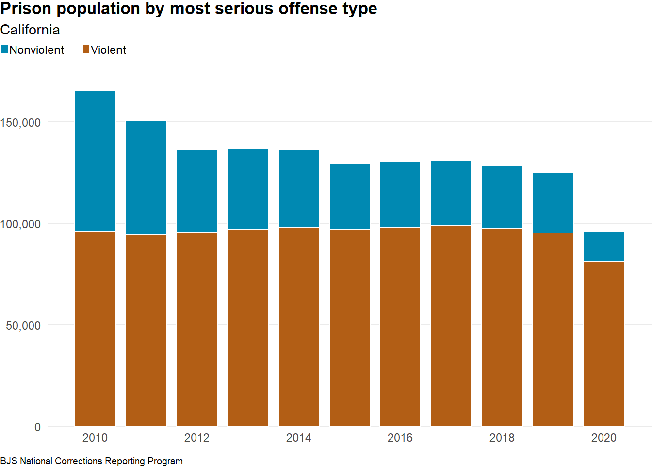
Save Image
Saving the image as a png file allows you to send the visualization to others or put the visualization into a presentation or documents. A crucial part of saving the image is establishing the size of the image that makes the visualization look the best.
ggsave(plot = gg_prison_population_by_offense,
filename = "img/gg_prison_population_by_offense.png", height = 2.7, width = 5.6)
Now the png file can be inserted into any file (shown below).

Create Dynamic Text from Data
We can also use the data to create text that reflects the change over time. Begin by setting the two years of interest (we will be looking at the change between the two years).
start_year <- 2010
end_year   <- 2020
With our years set, we can filter the already created data frame to only show the two years of interest. Then, rename the years from numbers (2010, 2020) to text. Now we can easily pivot the data frame to a wide format. We will put the values for start_year in one column and the values for end_year in another column.
prison_population_by_offense_wide <- toplot_state_prison_pop_offense_type |>
  # filter to only include the start year and end year
  filter(RPTYEAR %in% c(start_year, end_year)) |>
  mutate(RPTYEAR = case_when(
    RPTYEAR == start_year ~ "start_year",
    RPTYEAR == end_year   ~ "end_year"
  )) |>
  pivot_wider(names_from = RPTYEAR, values_from = n)
prison_population_by_offense_wide
#> # A tibble: 2 × 4
#> STATE violent_or_nonviolent start_year end_year
#> <chr> <chr> <dbl> <dbl>
#> 1 California Nonviolent 69147 14890
#> 2 California Violent 96096 81003Calculate the percentage change for both Nonviolent and Violent offense, and round the value to 2 digits. Next, we want to create specific text based on whether the percent change is positive or negative. We also add an option in case the percent change is 0. Finally, we order the data frame based on the percent change value. This will determine the order of sentences in the paragraph.
prison_population_by_offense_text <- prison_population_by_offense_wide |>
  mutate(pct_change = round( (end_year - start_year)/start_year, 2)) |>
  mutate(
    change_text = case_when(
      pct_change > 0 ~ paste0(
                              tolower(violent_or_nonviolent),
                              " offenses increased by ",
                              percent(pct_change, 1, suffix = " percent")
                              ),
      pct_change < 0 ~ paste0(
                              tolower(violent_or_nonviolent),
                              " offenses decreased by ",
                              percent(abs(pct_change), 1, suffix = " percent")
                              ),
      pct_change == 0 ~ "remained nearly the same"
    )
  ) |>
  arrange(pct_change)
prison_population_by_offense_text
#> # A tibble: 2 × 6
#> STATE violent_or_nonviolent start_year end_year pct_change change_text
#> <chr> <chr> <dbl> <dbl> <dbl> <chr>
#> 1 California Nonviolent 69147 14890 -0.78 nonviolent of…
#> 2 California Violent 96096 81003 -0.16 violent offen…Now that the prep work is completed, we can create the paragraph. We like using the glue() function to combine static and dynamic text.
Anything within curly brackets, {}, is run as code. Use 2 backslashes, \\, to specify that even though the code is continued on a new line there should NOT be line break in the paragraph. If the backslashes are removed, each time the code goes to a new line, there will be a line break in the paragraph.
prison_population_by_offense_paragraph <- glue(
    "Between {start_year} and {end_year} \\
    in {this_state}, the prison population serving sentences for \\
    {prison_population_by_offense_text$change_text[1]}, \\
    while the prison population serving sentences \\
    for {prison_population_by_offense_text$change_text[2]}."
)prison_population_by_offense_paragraphBetween 2010 and 2020 in California, the prison population serving sentences for nonviolent offenses decreased by 78 percent, while the prison population serving sentences for violent offenses decreased by 16 percent.
This code is great because we can create a new paragraph with different year inputs. Let’s say we want to look at the difference between 2015 and 2020. All we need to do is change the start_year to 2015 and the same code. Additionally, we are less likely to make mistakes because there are fewer manual tasks.
start_year <- 2015
end_year   <- 2020

prison_population_by_offense_text <- toplot_state_prison_pop_offense_type |>
  filter(RPTYEAR %in% c(start_year, end_year)) |>
  mutate(RPTYEAR = case_when(
    RPTYEAR == start_year ~ "start_year",
    RPTYEAR == end_year   ~ "end_year"
  )) |>
  pivot_wider(names_from = RPTYEAR, values_from = n) |>
  mutate(pct_change = round( (end_year - start_year)/start_year, 2)) |>
  mutate(
    change_text = case_when(
      pct_change > 0 ~ paste0(
                              tolower(violent_or_nonviolent),
                              " offenses increased by ",
                              percent(pct_change, 1, suffix = " percent")
                              ),
      pct_change < 0 ~ paste0(
                              tolower(violent_or_nonviolent),
                              " offenses decreased by ",
                              percent(abs(pct_change), 1, suffix = " percent")
                              ),
      pct_change == 0 ~ "remained nearly the same"
    )
  ) |>
  arrange(pct_change)

glue(
    "Between {start_year} and {end_year} \\
    in {this_state}, the prison population serving sentences for \\
    {prison_population_by_offense_text$change_text[1]}, \\
    while the prison population serving sentences \\
    for {prison_population_by_offense_text$change_text[2]}."
  )
Between 2015 and 2020 in California, the prison population serving sentences for nonviolent offenses decreased by 54 percent, while the prison population serving sentences for violent offenses decreased by 17 percent.
Average Length of Stay
Import Data
The data used for this visualization originally comes from the NCRP Prison Population dataset. If you are interested in downloading the NCRP data and cleaning it yourself, please review Appendix: NCRP Data.
state_los_url <- "https://raw.githubusercontent.com/CSGJusticeCenter/va_data/main/model_code/prison_pop_los/state_prison_avg_los.csv"
us_los_url <- "https://raw.githubusercontent.com/CSGJusticeCenter/va_data/main/model_code/prison_pop_los/us_prison_avg_los.csv"

state_prison_avg_los <- read_csv(state_los_url)
#> Rows: 11 Columns: 3
#> ── Column specification ────────────────────────────────────────────────────────
#> Delimiter: ","
#> chr (1): STATE
#> dbl (2): RELYR, mean
#>
#> ℹ Use `spec()` to retrieve the full column specification for this data.
#> ℹ Specify the column types or set `show_col_types = FALSE` to quiet this message.
us_prison_avg_los <- read_csv(us_los_url)
#> Rows: 11 Columns: 2
#> ── Column specification ────────────────────────────────────────────────────────
#> Delimiter: ","
#> dbl (2): RELYR, mean
#>
#> ℹ Use `spec()` to retrieve the full column specification for this data.
#> ℹ Specify the column types or set `show_col_types = FALSE` to quiet this message.

this_state <- state_prison_avg_los$STATE[1]
state_prison_avg_los
#> # A tibble: 11 × 3
#> STATE RELYR mean
#> <chr> <dbl> <dbl>
#> 1 California 2010 3.90
#> 2 California 2011 4.09
#> 3 California 2012 4.23
#> 4 California 2013 4.62
#> 5 California 2014 4.51
#> 6 California 2015 4.49
#> 7 California 2016 4.46
#> 8 California 2017 4.49
#> 9 California 2018 4.73
#> 10 California 2019 4.81
#> 11 California 2020 4.84us_prison_avg_los
#> # A tibble: 11 × 2
#> RELYR mean
#> <dbl> <dbl>
#> 1 2010 4.28
#> 2 2011 4.26
#> 3 2012 4.35
#> 4 2013 4.33
#> 5 2014 4.41
#> 6 2015 4.52
#> 7 2016 4.59
#> 8 2017 4.76
#> 9 2018 4.84
#> 10 2019 4.78
#> 11 2020 5.05Create Plot
Build ggplot
gg_prison_los_avg <- state_prison_avg_los |>
  ggplot(aes(
    x = RELYR,
    y = mean
  )) +
  geom_col(fill = "#6d6595", width = 0.8) +
  scale_x_continuous(breaks = seq(2010, 2020, by = 1)) + # set the report year to be integers
  scale_y_continuous(expand = expansion(mult= c(0, 0.05))) + # remove any add'l spacing on the bottom part of the y-axis
  labs(
    title = "Average length of stay (years) of people exiting prison",
    subtitle = paste0(this_state, ": Prison terms for violent offenses"),
    caption = "BJS National Corrections Reporting Program",
    x = NULL, # no x-axis label
    y = NULL  # no y-axis label
  ) +
  theme_minimal() +
  theme(
    plot.title = element_text(
      face = "bold", # make the title font bold
      margin = margin(0, 0, 5, 0) # add margin below title
    ),
    plot.subtitle = element_text(
      size = 11,
      margin = margin(0, 0, 10, 0)
    ),
    plot.caption = element_text(
      size = 7, # set the font size for caption
      margin = margin(10, 0, 0, 0), # add margin at top of caption
      hjust = 0 # make caption left-aligned
    ),
    plot.caption.position = "plot", # align caption to edge of plot
    plot.title.position = "plot", # align title to edge of plot
    axis.text = element_text(size = 9), # increase axis text
    panel.grid.major.x = element_blank(), # remove major grid lines from x-axis
    panel.grid.minor = element_blank(), # remove all minor grid lines from both x and y axis
    plot.margin = margin(1, 0, 0, 0), # remove almost all margin from plot
    legend.position = "top", # put legend at top of chart
    legend.justification = c(0, 0), # pul legend in top left corner
    legend.location = "plot", # align caption to edge of plot
    legend.key.size = unit(7.25, "pt"), # set the size of the boxes in legend
    legend.margin = margin(-5, 0, 5, 0), # specify margin for legend
    legend.box.spacing = unit(10, "pt"),
    legend.text = element_text(
      size = 9, # increase size of legend text
      margin = margin(0, 8, 0, 0) # set legend text margin
    ),
  )
gg_prison_los_avg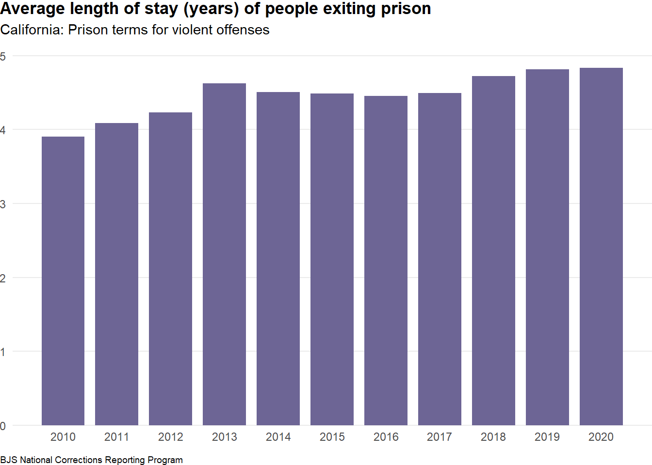
Save Image
Saving the image as a png file allows you to send the visualization to others or put the visualization into a presentation or documents.
ggsave(plot = gg_prison_los_avg,
  filename = "img/gg_prison_los_avg.png", height = 2.7, width = 5.6)
Now the png file can be inserted into any file (shown below).

Create Dynamic Text from Data
We can use the NCRP data to compare the mean length of stay for a specific state to the national value.
Start by specifying the year of interest (the last year data is available).
this_year <- 2020Next, we want to pull the national average length of stay for that year.
us_los_mean <- us_prison_avg_los |>
  filter(RELYR == this_year) |>
  pull(mean)
us_los_mean
#> [1] 5.046393Since we have the average national value for length of stay, we can calculate the percent change to the specific state length of stay.
We start by filtering the plot data to the specific year of interest and pulling out the mean length of stay.
state_los_mean <- state_prison_avg_los |>
  filter (RELYR == this_year) |>
  pull(mean)
state_los_mean
#> [1] 4.835823Next, we calculate the percent change compared to the U.S. value.
los_pct_diff <- (round(state_los_mean, 2) - round(us_los_mean, 2))/round(us_los_mean, 2)los_pct_diff
#> [1] -0.04158416Specify certain text depending on the percent change value.
pct_diff_text = if_else(
  los_pct_diff > 0,
  percent(abs(los_pct_diff), 1, suffix = " percent higher"),
  percent(abs(los_pct_diff), 1, suffix = " percent lower")
  )
pct_diff_text
#> [1] "4 percent lower"Finally, we can use the values we have calculated to create text within a paragraph.
prison_los_paragraph <- glue(
  "In {this_year}, the average length of stay of people released \\
   from prison who were serving time for a violent offense in {this_state} \\
   was {number(state_los_mean, 0.1)} years. This is {pct_diff_text} \\
   than the national average prison stay for violent offenses of \\
{number(us_los_mean, 0.1)} years.")prison_los_paragraphIn 2020, the average length of stay of people released from prison who were serving time for a violent offense in California was 4.8 years. This is 4 percent lower than the national average prison stay for violent offenses of 5.0 years.
R Session Info
#> ─ Session info ───────────────────────────────────────────────────────────────
#>  setting  value
#>  version  R version 4.4.2 (2024-10-31 ucrt)
#>  os       Windows 11 x64 (build 26100)
#>  system   x86_64, mingw32
#>  ui       RTerm
#>  language (EN)
#>  collate  English_United States.utf8
#>  ctype    English_United States.utf8
#>  tz       America/New_York
#>  date     2025-03-19
#>
#> ─ Packages ───────────────────────────────────────────────────────────────────
#>  ! package     * version date (UTC) lib source
#>  P bit           4.5.0.1 2024-12-03 []  CRAN (R 4.4.2)
#>  P bit64         4.5.2   2024-09-22 []  CRAN (R 4.4.2)
#>  P cli           3.6.3   2024-06-21 []  RSPM
#>  P colorspace    2.1-1   2024-07-26 []  CRAN (R 4.4.2)
#>  P crayon        1.5.3   2024-06-20 []  RSPM
#>  P curl          6.0.1   2024-11-14 []  RSPM
#>  P digest        0.6.37  2024-08-19 []  CRAN (R 4.4.2)
#>  P dplyr       * 1.1.4   2023-11-17 []  CRAN (R 4.4.2)
#>  P evaluate      1.0.1   2024-10-10 []  CRAN (R 4.4.2)
#>  P fansi         1.0.6   2023-12-08 []  CRAN (R 4.4.2)
#>  P farver        2.1.2   2024-05-13 []  CRAN (R 4.4.2)
#>  P fastmap       1.2.0   2024-05-15 []  CRAN (R 4.4.2)
#>  P forcats     * 1.0.0   2023-01-29 []  CRAN (R 4.4.2)
#>  P generics      0.1.3   2022-07-05 []  CRAN (R 4.4.2)
#>  P ggplot2     * 3.5.1   2024-04-23 []  CRAN (R 4.4.2)
#>  P glue        * 1.8.0   2024-09-30 []  RSPM
#>  P gtable        0.3.6   2024-10-25 []  CRAN (R 4.4.2)
#>  P hms           1.1.3   2023-03-21 []  CRAN (R 4.4.2)
#>  P htmltools     0.5.8.1 2024-04-04 []  CRAN (R 4.4.2)
#>  P htmlwidgets   1.6.4   2023-12-06 []  CRAN (R 4.4.2)
#>  P janitor     * 2.2.0   2023-02-02 []  CRAN (R 4.4.2)
#>  P jsonlite      1.8.9   2024-09-20 []  RSPM
#>  P knitr         1.49    2024-11-08 []  CRAN (R 4.4.2)
#>  P labeling      0.4.3   2023-08-29 []  CRAN (R 4.4.0)
#>  P lifecycle     1.0.4   2023-11-07 []  RSPM
#>  P lubridate   * 1.9.4   2024-12-08 []  CRAN (R 4.4.2)
#>  P magrittr      2.0.3   2022-03-30 []  RSPM
#>  P munsell       0.5.1   2024-04-01 []  CRAN (R 4.4.2)
#>  P pillar        1.9.0   2023-03-22 []  CRAN (R 4.4.2)
#>  P pkgconfig     2.0.3   2019-09-22 []  CRAN (R 4.4.2)
#>  P purrr       * 1.0.2   2023-08-10 []  RSPM
#>  P R6            2.5.1   2021-08-19 []  RSPM
#>  P ragg          1.3.3   2024-09-11 []  CRAN (R 4.4.2)
#>  P readr       * 2.1.5   2024-01-10 []  CRAN (R 4.4.2)
#>    renv          1.0.11  2024-10-12 []  CRAN (R 4.4.2)
#>  P rlang         1.1.4   2024-06-04 []  RSPM
#>  P rmarkdown     2.29    2024-11-04 []  CRAN (R 4.4.2)
#>  P scales      * 1.3.0   2023-11-28 []  CRAN (R 4.4.2)
#>  P sessioninfo   1.2.2   2021-12-06 []  CRAN (R 4.4.2)
#>  P snakecase     0.11.1  2023-08-27 []  CRAN (R 4.4.2)
#>  P stringi       1.8.4   2024-05-06 []  CRAN (R 4.4.0)
#>  P stringr     * 1.5.1   2023-11-14 []  CRAN (R 4.4.2)
#>  P systemfonts   1.1.0   2024-05-15 []  CRAN (R 4.4.2)
#>  P textshaping   0.4.1   2024-12-06 []  CRAN (R 4.4.2)
#>  P tibble      * 3.2.1   2023-03-20 []  CRAN (R 4.4.2)
#>  P tidyr       * 1.3.1   2024-01-24 []  CRAN (R 4.4.2)
#>  P tidyselect    1.2.1   2024-03-11 []  CRAN (R 4.4.2)
#>  P tidyverse   * 2.0.0   2023-02-22 []  CRAN (R 4.4.2)
#>  P timechange    0.3.0   2024-01-18 []  CRAN (R 4.4.2)
#>  P tzdb          0.4.0   2023-05-12 []  CRAN (R 4.4.2)
#>  P utf8          1.2.4   2023-10-22 []  CRAN (R 4.4.2)
#>  P vctrs         0.6.5   2023-12-01 []  RSPM
#>  P vroom         1.6.5   2023-12-05 []  CRAN (R 4.4.2)
#>  P withr         3.0.2   2024-10-28 []  RSPM
#>  P xfun          0.49    2024-10-31 []  CRAN (R 4.4.2)
#>  P yaml          2.3.10  2024-07-26 []  RSPM
#>
#>
#>  P ── Loaded and on-disk path mismatch.
#>
#> ──────────────────────────────────────────────────────────────────────────────
Appendix: NCRP Data
This appendix describes how to download the NCRP datasets and the code used to build the datasets used to create the visualizations shown above.
Download NCRP Data and Import
Start by making an ICPSR account.
After your account is set up, go to the National Corrections Reporting Program, 1991-2020: Selected Variables webpage. Select the second tab labeled “Data & Documentation.” Download both the “DS3 Prison Releases” and “DS4 Year-end Population.” Click the download button and select “R” to download the .rda files.
The R files are called 38492-0003-Data.rda and 38492-0004-Data.rda.
Next, load the data using the code below.
load("data/38492-0003-Data.rda")
load("data/38492-0004-Data.rda")
After loading the datasets, they will be listed in your environment. Notice that the names of the datasets are different than the file names.
Select a State
The visualizations shown above are designed to display data for a single state, so our first step is pick a state.
this_state <- "California" # select statePrison Population Data Prep
state_prison_pop_offense_type <- da38492.0004 |>
  mutate(STATE = str_sub(STATE, 6, -1)) |>  # remove the fips code from the state identifier
  filter(STATE == this_state, RPTYEAR >= 2010) |> # filter to specific state and report years
  as_tibble() |> # make the data frame a tibble
  mutate( # create a new variable that determines if offense is violent or non-violent
    violent_or_nonviolent = case_when(
      OFFGENERAL == "(1) Violent" ~ "Violent",
      is.na(OFFGENERAL) ~ NA_character_,
      TRUE ~ "Nonviolent"
  )) |>
  group_by(STATE, RPTYEAR, violent_or_nonviolent) |> # set the groupings for counts
  count() |> # count up the number of observations (rows) for each grouping
  ungroup() # remove group variables
state_prison_pop_offense_type
#> # A tibble: 33 × 4
#> STATE RPTYEAR violent_or_nonviolent n
#> <chr> <dbl> <chr> <int>
#> 1 California 2010 Nonviolent 69147
#> 2 California 2010 Violent 96096
#> 3 California 2010 <NA> 56
#> 4 California 2011 Nonviolent 56119
#> 5 California 2011 Violent 94198
#> 6 California 2011 <NA> 163
#> 7 California 2012 Nonviolent 40741
#> 8 California 2012 Violent 95319
#> 9 California 2012 <NA> 144
#> 10 California 2013 Nonviolent 39943
#> # ℹ 23 more rowsPrison Releases (Length of Stay) Data Prep
state_prison_avg_los <- da38492.0003 |>
  mutate(STATE = str_sub(STATE, 6, -1)) |>  # remove the fips code from the state identifier
  filter(STATE == this_state, RPTYEAR >= 2010) |> # filter to specific state and report years
  as_tibble() |> # make the data frame a tibble
  filter(
    SENTLGTH != "(0) < 1 year", # remove observations that have a sentence length less than a year
    ADMTYPE == "(1) New court commitment", # only look at new court commitments
    !is.na(RELYR),  # remove observations that don't have a release year
    OFFGENERAL == "(1) Violent" # only look at violent offenses
  ) |>
  mutate(los = RELYR - ADMITYR) |> # calculate length of stay (in years)
  group_by(STATE, RELYR) |>
  summarise(
    mean = mean(los),
    .groups = "drop" # drop groups (RELYR) after calculate summary
  )
state_prison_avg_los
#> # A tibble: 11 × 3
#> STATE RELYR mean
#> <chr> <dbl> <dbl>
#> 1 California 2010 3.90
#> 2 California 2011 4.09
#> 3 California 2012 4.23
#> 4 California 2013 4.62
#> 5 California 2014 4.51
#> 6 California 2015 4.49
#> 7 California 2016 4.46
#> 8 California 2017 4.49
#> 9 California 2018 4.73
#> 10 California 2019 4.81
#> 11 California 2020 4.84us_prison_avg_los <- da38492.0003 |>
filter(
SENTLGTH != "(0) < 1 year", # remove observations that have a sentence length less than a year
ADMTYPE == "(1) New court commitment", # only look at new court commitments
RELYR >= 2010, # pull all data that is 2010 or later
OFFGENERAL == "(1) Violent", # only look at violent offenses
) |>
mutate(los = RELYR - ADMITYR) |>
group_by(RELYR) |>
summarize(mean = mean(los, na.rm = TRUE))us_prison_avg_los
#> # A tibble: 11 × 2
#> RELYR mean
#> <dbl> <dbl>
#> 1 2010 4.28
#> 2 2011 4.26
#> 3 2012 4.35
#> 4 2013 4.33
#> 5 2014 4.41
#> 6 2015 4.52
#> 7 2016 4.59
#> 8 2017 4.76
#> 9 2018 4.84
#> 10 2019 4.78
#> 11 2020 5.05